install.packages("RMySQL")

library(DBI)
library(RMySQL)
library(here)

SQL_Con <- dbConnect(RMySQL::MySQL(), dbname = 'data_diabetes_RStudio', username = 'root', host='localhost', password = 'Chism1154')Data7 Exploratory Data Analysis in MySQL

Purpose of Materials
Exploratory data analysis of a novel data set with MySQL
Objectives
- Load and explore a data set with summary statistics
- Diagnose and remove outliers
- Diagnose missing values in a data set
Overview
Exploratory data analysis is an essential first step towards determining the validity of your data and should be performed throughout the data pipeline. However, EDA is often performed too late or not at all.
SQL (Structured Query Language) is a programming language for database management, which lets you store, retrieve, manage, and manipulate data tables within databases. Though SQL has limited mathematical capabilities it can be used to perform EDA. A major disadvantage however is that SQL cannot be used to perform statistical graphics and other data visualization methods. For this, I recommend either the R programming language, specifically through the RStudio IDE and ggplot2 from the tidyverse package suite, or Python, specifically the seaborn library.
Here, we utilize MySQL to conduct preliminary exploratory data analysis aimed at diagnosing any major issues with an imported data set. We introduce a clean and straightforward methodology to uncover issues such as data outliers, missing data, as well as summary statistical reports.
Required Setup
We first need to prepare our environment with the necessary libraries and start our MySQL connection. Note that you can use SQLite for some of these functions, but not all.
Examine and Describe a Data Set
- Examine columns and data types
- Summary statistics
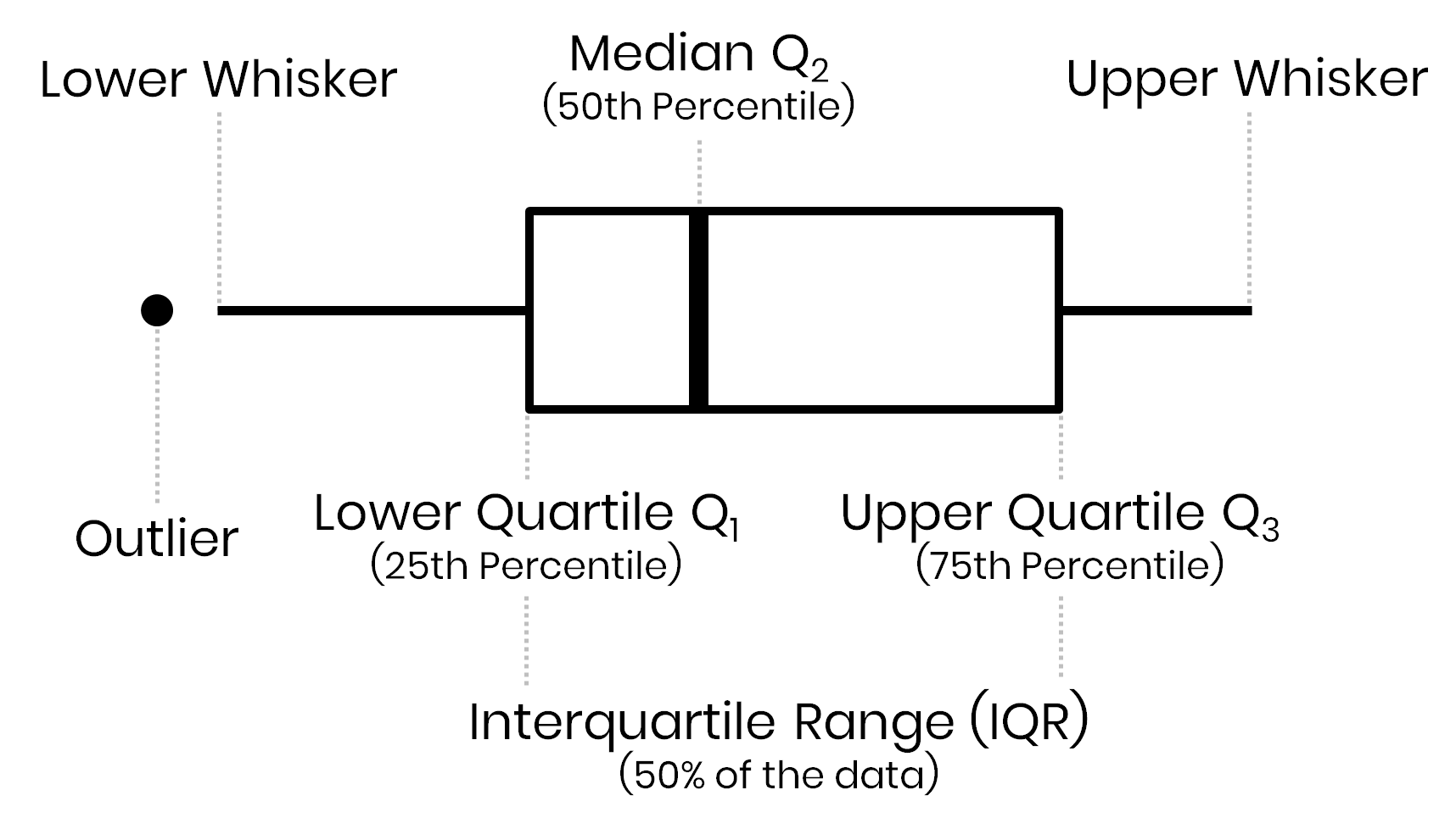
- Define box plots
- Describe meta data
Examine a Data Set
We should always examine a dataset in our databases. Here we are looking at the first 5 rows of the dataset.
-- First 5 rows
SELECT *
FROM diabetes
LIMIT 5;| Pregnancies | Glucose | BloodPressure | SkinThickness | Insulin | BMI | DiabetesPedigreeFunction | Age | Outcome |
|---|---|---|---|---|---|---|---|---|
| 6 | 148 | 72 | 35 | 0 | 33.6 | 0.627 | 50 | 1 |
| 1 | 85 | 66 | 29 | 0 | 26.6 | 0.351 | 31 | 0 |
| 8 | 183 | 64 | 0 | 0 | 23.3 | 0.672 | 32 | 1 |
| 1 | 89 | 66 | 23 | 94 | 28.1 | 0.167 | 21 | 0 |
| 0 | 137 | 40 | 35 | 168 | 43.1 | 2.288 | 33 | 1 |
Describe your Data
We need to start by seeing what data types our columns actually are.
-- What are the properties of the data
DESCRIBE diabetes;| Field | Type | Null | Key | Default | Extra |
|---|---|---|---|---|---|
| Pregnancies | int | YES | NA | ||
| Glucose | int | YES | NA | ||
| BloodPressure | int | YES | NA | ||
| SkinThickness | int | YES | NA | ||
| Insulin | int | YES | NA | ||
| BMI | double | YES | NA | ||
| DiabetesPedigreeFunction | double | YES | NA | ||
| Age | int | YES | NA | ||
| Outcome | int | YES | NA |
Field: name of each variabletype: data type of each variableNull: allows NULL valuesKey: primary key that was usedDefault: default value for the columnExtra: any additional information
Unique values
Next we can look at unique values within columns - e.g., Pregnancies and Age.
SELECT
DISTINCT Pregnancies, Age
FROM diabetes;| Pregnancies | Age |
|---|---|
| 6 | 50 |
| 1 | 31 |
| 8 | 32 |
| 1 | 21 |
| 0 | 33 |
| 5 | 30 |
| 3 | 26 |
| 10 | 29 |
| 2 | 53 |
| 8 | 54 |
Filtering
We can also filter data by qualifications.
SELECT *
FROM diabetes
WHERE Age >= 50
LIMIT 5;| Pregnancies | Glucose | BloodPressure | SkinThickness | Insulin | BMI | DiabetesPedigreeFunction | Age | Outcome |
|---|---|---|---|---|---|---|---|---|
| 6 | 148 | 72 | 35 | 0 | 33.6 | 0.627 | 50 | 1 |
| 2 | 197 | 70 | 45 | 543 | 30.5 | 0.158 | 53 | 1 |
| 8 | 125 | 96 | 0 | 0 | 0.0 | 0.232 | 54 | 1 |
| 10 | 139 | 80 | 0 | 0 | 27.1 | 1.441 | 57 | 0 |
| 1 | 189 | 60 | 23 | 846 | 30.1 | 0.398 | 59 | 1 |
Sorting
We might want to sort columns in ascending (ASC) or descending (DESC) order.
SELECT Glucose, Age
FROM diabetes
ORDER BY Glucose ASC
LIMIT 10;| Glucose | Age |
|---|---|
| 0 | 41 |
| 0 | 21 |
| 0 | 22 |
| 0 | 37 |
| 0 | 22 |
| 44 | 36 |
| 56 | 22 |
| 57 | 67 |
| 57 | 41 |
| 61 | 46 |
Summary Statistics of your Data
Numerical Variables
Our entire database is numerical data, but we will look at two of the numerical columns, Glucose and Insulin.
Note that the stat column will be called ‘Count’ but this isn’t a problem.
-- Summary statistics of our numerical columns
SELECT 'Count',
    count(Glucose) as Glucose,
    count(Insulin) as Insulin
FROM diabetes
UNION
SELECT 'Total',
    sum(Glucose) as Glucose,
    sum(Insulin) as Insulin
FROM diabetes
UNION
SELECT 'Mean',
    avg(Glucose),
    avg(Insulin)
FROM diabetes
UNION
SELECT 'Min',
    min(Glucose),
    min(Insulin)
FROM diabetes
UNION
SELECT 'Max',
    max(Glucose),
    max(Insulin)
FROM diabetes
UNION
SELECT 'Std. Dev.',
    STDDEV_SAMP(Glucose),
    STDDEV_SAMP(Insulin)
FROM diabetes
UNION
SELECT 'Variance',
    VAR_SAMP(Glucose),
    VAR_SAMP(Insulin)
FROM diabetes; | Count | Glucose | Insulin |
|---|---|---|
| Count | 768.00000 | 768.00000 |
| Total | 92847.00000 | 61286.00000 |
| Mean | 120.89453 | 79.79948 |
| Min | 0.00000 | 0.00000 |
| Max | 199.00000 | 846.00000 |
| Std. Dev. | 31.97262 | 115.24400 |
| Variance | 1022.24831 | 13281.18008 |
Count: number of observationsTotal: sum of all values in a columnsMean: arithmetic mean (average value)Min: minimum valueMax: maximum valueStd. Dev.: standard deviation of the dataVariance: variance of the data
Median and Percentiles
SQL does not have straightforward functions for percentiles (including the Median), so let’s write them!
Make 100 bins
Assign percentiles to bins
Select desired percentiles (25, 50, 75) = (Q1, Median, Q3)
WITH perc AS (SELECT Glucose, NTILE(100) OVER (ORDER BY Glucose) AS 'Percentile'
FROM diabetes)
SELECT Percentile, MAX(Glucose) as Glucose
FROM perc
GROUP BY Percentile
HAVING Percentile = 25 OR Percentile = 50 or Percentile = 75;| Percentile | Glucose |
|---|---|
| 25 | 100 |
| 50 | 119 |
| 75 | 144 |
Categorical Variables
Our original data does not have a categorical column, so we will use diabetes_Age. In the Age_group column categories were created by a qualifier:
Young: Age <= 21
Middle: Age between 21 and 30
Elderly: Age > 30
SELECT Age_group,
       COUNT(*) AS 'Count',
       COUNT(*) * 1.0 / SUM(COUNT(*)) OVER () AS 'Ratio'
FROM diabetes_Age
GROUP BY Age_group| Age_group | Count | Ratio |
|---|---|---|
| Middle | 270 | 0.35156 |
| Young | 417 | 0.54297 |
| Elderly | 81 | 0.10547 |
Count: number of values in the columnRatio: the number of observations over the total observations
Outliers
Values outside of \(1.5 * IQR\)
There are several numerical variables that have outliers above, let’s see what the data look like with and without them.
Outlier Detection
The most common method to detect outliers is by using the interquartile range:
\(1.5 * IQR\). Above we found the first and third quartiles for Glucose (Q1 = 100, Q3 = 144), therefore the IQR is 44.
Qualifier: \(1.5∗44=66\)
Lower limit: \(100-66 = 34\)
Upper limit: \(144 + 66 = 210\)
SELECT Glucose
FROM diabetes
WHERE Glucose < 210 AND Glucose > 34
ORDER BY Glucose ASC;| Glucose |
|---|
| 44 |
| 56 |
| 57 |
| 57 |
| 61 |
| 62 |
| 65 |
| 67 |
| 68 |
| 68 |
Missing Values (NAs)
Table showing the extent of NAs in columns containing them.
SELECT *
FROM
diabetesNA
LIMIT 5;| Pregnancies | Glucose | BloodPressure | SkinThickness | Insulin | BMI | DiabetesPedigreeFunction | Age | Outcome |
|---|---|---|---|---|---|---|---|---|
| 6 | 148 | 72 | 35 | NA | 33.6 | 0.627 | 50 | NA |
| 1 | NA | NA | NA | 0 | NA | 0.351 | 31 | 0 |
| 8 | 183 | 64 | NA | 0 | 23.3 | 0.672 | 32 | 1 |
| NA | 89 | NA | 23 | NA | 28.1 | 0.167 | NA | 0 |
| NA | 137 | 40 | 35 | NA | 43.1 | 2.288 | 33 | 1 |
However, “NA” is not NULL in SQL, so we will have to change this.
- Create new table from diabetesNA.
CREATE TABLE diabetesNull
AS
SELECT *
FROM diabetesNA;- Change
'NA'intoNULL- Its possible to do this all in one argument, but I find that temperamental.
Pregnancies
UPDATE diabetesNull
SET
Pregnancies = NULL WHERE Pregnancies = 'NA';
Glucose
UPDATE diabetesNull
SET
Glucose = NULL WHERE Glucose = 'NA';
BloodPressure
UPDATE diabetesNull
SET
BloodPressure = NULL WHERE BloodPressure = 'NA';
SkinThickness
UPDATE diabetesNull
SET
SkinThickness = NULL WHERE SkinThickness = 'NA';
Insulin
UPDATE diabetesNull
SET
Insulin = NULL WHERE Insulin = 'NA';
BMI
UPDATE diabetesNull
SET
BMI = NULL WHERE BMI = 'NA';
DiabetesPedigreeFunction
UPDATE diabetesNull
SET
DiabetesPedigreeFunction = NULL WHERE DiabetesPedigreeFunction = 'NA';
Age
UPDATE diabetesNull
SET
Age = NULL WHERE Age = 'NA';
Outcome
UPDATE diabetesNull
SET
Outcome = NULL WHERE Outcome = 'NA';
Diagnose NAs
Now we can see true NAs! (They look the same in the Quarto render, but SQL treats them differently)
SELECT *
FROM diabetesNULL | Pregnancies | Glucose | BloodPressure | SkinThickness | Insulin | BMI | DiabetesPedigreeFunction | Age | Outcome |
|---|---|---|---|---|---|---|---|---|
| 6 | 148 | 72 | 35 | NA | 33.6 | 0.627 | 50 | NA |
| 1 | NA | NA | NA | 0 | NA | 0.351 | 31 | 0 |
| 8 | 183 | 64 | NA | 0 | 23.3 | 0.672 | 32 | 1 |
| NA | 89 | NA | 23 | NA | 28.1 | 0.167 | NA | 0 |
| NA | 137 | 40 | 35 | NA | 43.1 | 2.288 | 33 | 1 |
| 3 | 78 | 50 | 32 | NA | 31 | 0.248 | 26 | 1 |
| NA | 115 | 0 | 0 | 0 | NA | 0.134 | NA | 0 |
| 2 | 197 | 70 | NA | 543 | 30.5 | 0.158 | 53 | NA |
| 4 | NA | NA | NA | 0 | NA | 0.191 | 30 | 0 |
| 10 | 168 | 74 | 0 | 0 | 38 | 0.537 | 34 | 1 |
We can see the number of NULL values in each column.
SELECT 'NAs',
    SUM(CASE WHEN Glucose IS NULL THEN 1 ELSE 0 END) AS Glucose,
    SUM(CASE WHEN Insulin IS NULL THEN 1 ELSE 0 END) AS Insulin
FROM diabetesNULL
UNION
SELECT 'NA Freq',
    SUM(CASE WHEN Glucose IS NULL THEN 1 ELSE 0 END) / SUM(CASE WHEN Glucose IS NULL THEN 0 ELSE 1 END) AS Glucose,
    SUM(CASE WHEN Insulin IS NULL THEN 1 ELSE 0 END) / SUM(CASE WHEN Insulin IS NULL THEN 0 ELSE 1 END) AS Insulin
FROM diabetesNULL| NAs | Glucose | Insulin |
|---|---|---|
| NAs | 168.0000 | 164.0000 |
| NA Freq | 0.4541 | 0.4385 |
Created: 09/21/2022 (G. Chism); Last update: 09/21/2022
